Particle Swarm Optimization on Heston Small-Time Expansion
Here, I look at the problem of calibrating a Heston small-time expansion, the one from Forde & Jacquier. This can be useful to find a good initial guess for the exact Heston calibration, computed with much costlier characteristic function Fourier numerical integration. I conclude with the madness of the life science inspired optimizers…
July 6, 2017
This is a sequel to my previous post on Particle Swarm Optimization. Here, I look at the problem of “calibrating” a Heston small-time expansion, the one from Forde & Jacquier). This can be useful to find a good initial guess for the exact Heston calibration, computed with much costlier characteristic function Fourier numerical integration.
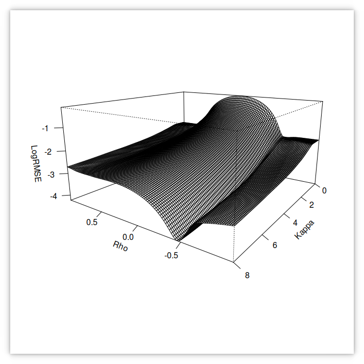
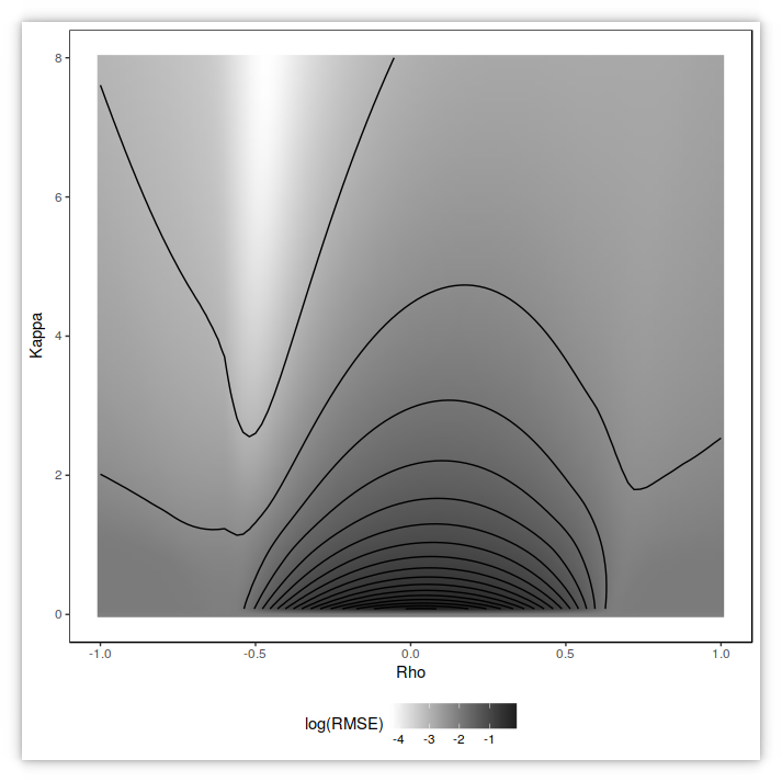
Unfortunately, as we see below, with the contour plots of the objective function
(the RMSE in volatilities against market quotes), the problem is much less well behaved with the small-time expansion
than with the numerical integration.
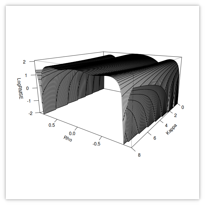
RMSE of the small-time Heston implied volatilities against SPX500 options volatilities in 1995 using v_0=0.009527, theta= 0.02318, sigma= 0.92745 and varying kappa and rho.
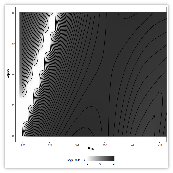
contour plot of the small-time RMSE
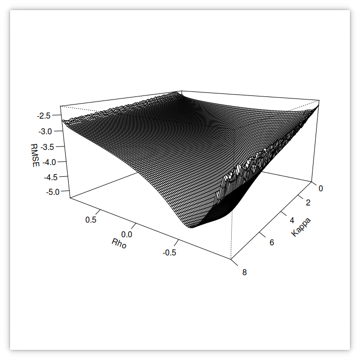
RMSE of the Fourier-based Heston implied volatilities against SPX500 options volatilities in 1995 using v_0=0.009527, theta= 0.02318, sigma= 0.92745 and varying kappa and rho.
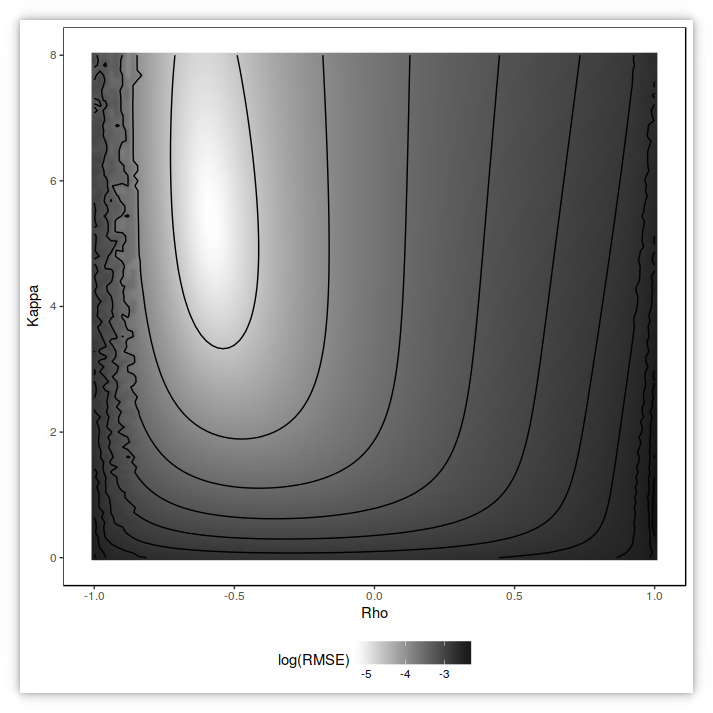
contour plot of the Fourier-based (nearly exact) RMSE
In deed, with the small-time expansion, the Heston parameters have no particular meaning beyond the range where the small-time expansion is valid. Used outside it creates spurious interdependencies. Filtering out quotes helps but is not enough to strongly stabilize the problem, unless we calibrate against only two option maturities. The expansion from Forde has actually an analytical solution from 4 points on two maturities plus an initial variance estimate, and a global calibration of the small-time expansion on two expiries is thus not very useful.
Still, it provides a good test of global minimizers, as the objective function has many local minima. By filtering out some quotes, we create slightly different calibration problems which can be more or less challenging that the unfiltered problem. In order to assess the flexibility of differential evolution (DE), simulated annealing (SA) and particle swarm optimization (PSO), we look at 12 different problems:
- option quotes in 1995 and in 2010,
- using a root mean square error (RMSE) measure in volatilities or an inverse vega weighted RMSE in prices,
- with no filtering, or filtering out market quotes with a normalized price less than 1E-6, or filtering out market quotes corresponding to options of longer maturity than 1 year or larger log-moneyness than 20%.
Then we compute the number of calibration failures. A failure corresponds to a L2-distance of the Heston parameters from the true minimum larger than 0.1, ignoring the kappa. This is in general more representative than the distance in RMSE as two close RMSEs can stem from quite different parameters if those correspond to two different local minima.
As all the global minimizers considered rely on random numbers, they will produce different results depending on the initial seed used for random number generation. It is then entirely possible that a specific minimizer will perform very well by luck, but with another choice of seed, it might not perform as well. In order to remove this bias, I run 50 minimizations with different seeds (I jump to a far away point 100 times instead of simply picking 100 different random seeds) and compute the mean and the standard error for each minimizer.
I consider different settings for each minimizer. The table below shows the best contenders among many different settings tried.
| Minimizer | Mean failures (Std error) | Min | Max |
|---|---|---|---|
| DE NP=30 F=0.8 CR=0.6 Rand1EitherOr | 1.54 (0.10) | 1 | 4 |
| DE NP=30 F=0.7 CR=0.7 Rand1Bin | 2.84 (0.10) | 2 | 5 |
| DE NP=30 F=0.8 CR=0.7 Best1Bin | 3.74 (0.15) | 1 | 6 |
| SA T=1 RT=0.8 NS=4 NT=20 | 2.02 (0.13) | 0 | 5 |
| PSO S=100 von Neumann c1=c2=2.02 PhiEnd=2*2.2 | 2.72 (0.13) | 1 | 5 |
| PSO S=81 von Neumann c1=c2=2.02 PhiEnd=2*2.2 | 3.00 (0.16) | 1 | 5 |
| PSO S=49 von Neumann c1=c2=2.02 PhiEnd=2*2.2 | 3.84 (0.16) | 2 | 6 |
In the PSO, the particle can go beyond the boundaries, what to do then?
- stick the particle at the boundary if it goes beyond and set the velocity to zero (Nearest-Z). This is recommended in Clerc’s book but led to the highest failure rate on average.
- ignore the particles that move beyond the boundary in the calculation of the best positions (Infinity). This is the choice of the standard PSO 2007. It produced a much smaller failure rate on average.
- reflect the particle at the boundary and set its velocity to zero (Reflect-Z). This led to the smallest failure rate on average, which confirms the findings of the paper “Analyzing the Effects of Bound Handling in Particle Swarm Optimization”.
| Minimizer | Mean failures (Std error) | Min | Max |
|---|---|---|---|
| Reflect-Z with S=100 | 2.46 (0.12) | 1 | 4 |
| Reflect-Z with S=81 | 2.54 (0.13) | 1 | 5 |
| Infinity with S=100 | 2.72 (0.13) | 1 | 5 |
| Infinity with S=81 | 3.00 (0.16) | 1 | 5 |
| Nearest-Z with S=100 | 3.04 (0.15) | 1 | 6 |
| Nearest-Z with S=81 | 3.42 (0.17) | 1 | 6 |
PSO is not only less robust in general, it is also slower with the settings chosen (a smaller swarm size would increases the failures even more). Here is a table with the time needed to calibrate the minimizers with the best settings above against all the quotes in 1995:
| Minimizer | Time(ms) |
|---|---|
| DE Best1Bin | 156 |
| DE Rand1EitherOr | 267 |
| DE Rand1Bin | 314 |
| SA | 427 |
| PSO S=100 | 581 |
| PSO S=81 | 790 |
| PSO S=49 | 378 |
The time is however only indicative since it will be highly dependent on the stopping criteria, and each method use a different stopping criteria.
Matt Lorig et al. provide two different small-time Heston expansions of order 2 and 3. Interestingly, they behave quite well on our example as evidenced by the 3d graph and the contour plot of
the RMSE below.
RMSE of the small-time Heston implied volatilities against SPX500 options volatilities in 1995 using v_0=0.009527, theta= 0.02318, sigma= 0.92745 and varying kappa and rho.
contour plot of the small-time RMSE
The global minimizers can then use more agressive settings, that is ones that will converge faster (with the risk of being stuck in a local minimum more frequently).
| Minimizer | Mean failures (Std error) | Min | Max |
|---|---|---|---|
| DE NP=15 F=0.9 CR=0.5 Best1Bin | 0.24 (0.07) | 0 | 2 |
| SA T=1 RT=0.9 NS=3 NT=15 | 0.28 (0.06) | 0 | 1 |
| PSO S=49 von Neumann c1=c2=2.02 PhiEnd=4.4 | 0.08 (0.04) | 0 | 1 |
To conclude, PSO can work to calibrate Heston even if it tends to struggle on more complex problems. I however found differential evolution and to some extent simulated annealing more intuitive, more easily tweaked, and better performing.
The life science that James Kennedy (a psychologist) introduced with the PSO is extremely fashionable these days. Anyone seems to create their own algorithm based on some dubious life science analogy. Papers on this get published and you end up with crap algorithms like the firefly algorithm with more than 800 citations! Among those you can find: the grey wolf optimization, the flower pollination algorithm, the cuckoo search, the ant lion optimizer, the whale optimization algorithm, the bat algorithm, the elephant herding optimization… And I am not making those up!
Don’t waste your time on those. I could not obtain any decent result from the firefly algorithm (the basic algorithm with the constant random factor looks very suspicious anyway), not surprising that its inventor is linked to the Allais effect, which looks like a good scam, even if the Allais paradox is interesting.