The Fastest Implied Volatility Algorithms, Go vs. Julia
In the second edition of my book, I presented how to combine the good Black-Scholes implied volatility initial guess of Dan Stefanica and Rados Radoicic with a relatively simple solver. Here, I present how to further enhance the performance, and compare as well implementations in the Go language vs. the Julia language.
December 2, 2020
In my book, I took a close look at the idea presented in the Chase the Devil blog to combine the very good initial Black-Scholes implied volatility guess of Dan Stefanica and Rados Radoicic with a relatively simple solver. The blogger recently criticized some new book, which clumsily tries to sell that idea as a novel algorithm, and presents fully inconsistent timing to assert that his new algorithm is much better.
The first important question is: why would we care about a fast and very accurate implied volatility solver?
Indeed, the market quotes prices which can not be too small. If the goal is to invert those, it would seem at first that the accuracy required would correspond to the smallest quoted price increment (1 cent or more precisely, 1 tick). Of course, this is absolute prices, and relative to the asset price, the accuracy should perhaps be around 0.0001.
This view misses the main point. When a model is fitted against market prices, the model may produce arbitrarily small prices, typically in the wings. It is not uncommon to fit in terms of implied volatilities, perhaps because it is a more natural scale along expiries and strikes, perhaps because of traders bias towards looking at the market in terms of implied volatilities. Those very small prices will need to be inverted, if the error measure is in implied volatilities. Furthermore, even in the nicer at-the-money region, the calibration of the model will likely involve differentiation of the outputs towards the inputs. If the implied volatility algorithm is unprecise, this will create a lot of numerical noise, and the calibration may easily be trapped in some local minima.
Go vs. Julia
Go feels like a low level programming language compared to Julia. When porting Peter Jaeckel algorithm for the implied volatility to Julia, there was the need to also port the related code: the cumulative normal distribution, erfcx from Cody and the inverse cumulative normal distribution from Wichura. It may be possible to find some of those in some Go open-source libraries, but perhaps not with the degree of accuracy or robustness desired.
In Julia, I could just use the SpecialFunctions package, which is maintained by top academic experts. Out of curiosity, I also ported the exact same code as in my Go implementation. Here is the timing I measured on the example of a Call option price with forward price of 100.0, strike of 300.0, vol of 8% (using Julia BenchmarkTools and go benchmark):
| Julia | Julia (Cody) | Go |
|---|---|---|
| 827.813 ns | 874.890 ns | 919 ns |
The default Julia implementation is faster than the specialized algorithms of Cody and Wichura referenced by Jaeckel implementation. On the same machine, Julia ends up thus around 10% faster than Go on this example.
Alternative Algorithms
Next, I wondered how my Householder implementation on top of the good initial guess would fare with the Julia libraries. A key performance improvement is to not rely on the naive Black-Scholes implementation via the cumulative normal distribution, but to use Peter Jaeckel expression in terms of erfcx. This speeds up the algorithms by 30-40%.
Another even more important trick is to apply the iteration on the logarithm of the option price. I noticed this, as I was experimenting with multiple precision support, and it turns out that for very low volatility, when the price is extremely small, Householder is very slow to converge. This can be seen in the plot below where it seems to take an exponentially longer time for very low volatilities.
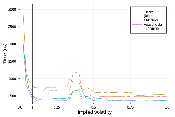
Time to imply the volatility from a 1y option of strike 200, forward 100, varying the reference vol.
Taking the log makes a tremendous difference:
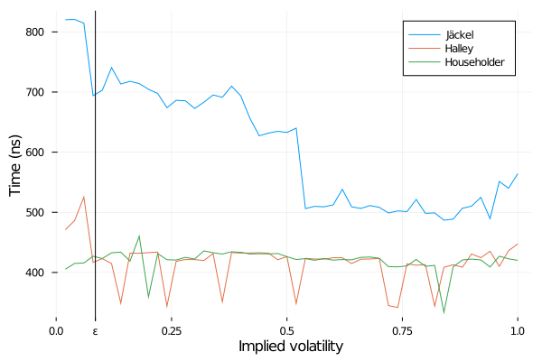
Time to imply the volatility from a 1y option of strike 200, forward 100, varying the reference vol - using log price.
The epsilon above denotes the limit at which the price is under machine epsilon. The timing, varying the strike, for a fixed vol is as good:
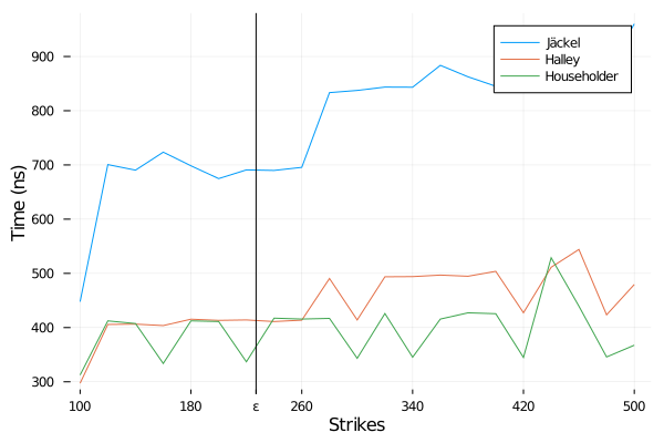
Time to imply the volatility from a 1y option of forward 100, vol=10%, varying the option strike - using log price.
So far, Halley is almost as fast as Householder, this is not true anymore if we look at a fixed high vol (400%):
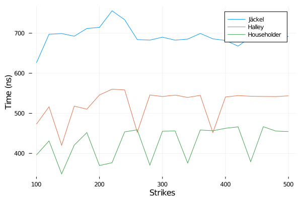
Time to imply the volatility from a 1y option of forward 100, vol=400%, varying the option strike - using log price.
Peter Jaeckel algorithm is then always slower. So it is not so difficult to write a much simpler, and faster algorithm. There is a place however where Peter Jaeckel really took a lot of care, it is to ensure a maximum accuracy, even in corner cases. My simple Householder algorithm “only” achieves an accuracy of around 1E-14 in implied volatility for a Call option of strike 200.0 and volatility 400%, while Peter Jaeckel algorithm pushes that up to 4E-15. In this case, Householder is within 2 machine epsilon accuracy in terms of price, while Jaeckel is within 1 machine epsilon accuracy.
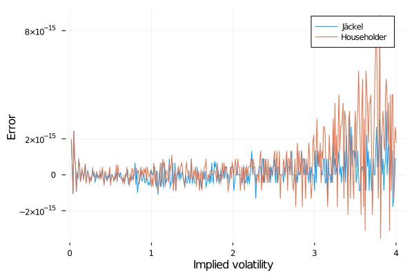
Error in the implied volatility from a 1y option of strike 200, forward 100, varying the reference vol.
As an extra bonus of working in Julia, the code can also make use of multiple or arbitrary precision arithmetic to reach any desired accuracy level, even if the use cases for this are very rare.
I am planning to put the associated Julia code on github, along with other illustrative examples from my book.