Julia and Python for the RBF collocation of a 2D PDE with multiple precision arithmetic
This is not going to be a comparison between Julia and Python in general. I am sure there exists already many great articles on Julia vs. XYZ language available on the internet. The below is more a hands on Julia from a numerical scientist point of view, when applied to the RBF collocation of a 2D PDE.
May 24, 2019
I was curious about using Julia, mainly to access the Arb library for arbitrary precision linear algebra. It is written by the author of Python mpmath library, but its principle is quite different, and from the author’s blog, it is supposed to be much faster. Then, I also found python + numpy + scipy not so great at building large sparse matrices. It seemed relatively slow to me, numba does not work with scipy sparse matrices. Numba is in general not so nice to use, except to inline some very simple function. So I had previously thought of moving some of my code to Julia. Those remarks should be taken with a grain of salt, because I am no expert in numpy, scipy or numba.
The problem I solved is closely linked to the solution of the Heston 2D-PDE. I was sort of curious to see if RBF collocation was any good, and what was its performance in practice. Compared to a classic finite difference discretization, the RBF collocation implies the solution of dense matrices instead of sparse (usually tridiagonal) matrices. One may need however much less discretization points to achieve a reasonable accuracy with the collocation approach.
The RBF collocation function is $$ f(x) = \sum_{i=1}^{n} a_j \sqrt{c^2 + \Vert x - x_i \Vert^2} $$
where c is called the shape parameter. The points x are in the two dimensional space and correspond to the spot and variance (S,v) of the Heston model. I used a simple rectangular grid.
One notable issue of RBF interpolation (with a multiquadric function or some other infinite support function) is that the resulting linear system may be ill-conditioned when c is too large (the multiquadric function behaves then almost like an affine function), due to the limits of the double number representation (64-bits). But how large is too large? What is a good choice for c? Those are difficult questions.
A recent paper from Kansa, titled On the ill-conditioned nature of RBF strong collocation, suggests that a large c is often optimal (note that the RBF is sometimes expressed with \( \epsilon=\frac{1}{c} \), also called shape parameter, and this paper is very ambiguous about the notation), as long as we use multiple precision arithmetic, for example floats on 256 bits. This is why I thought of trying, at first the mpmath library, until I stumbled upon the Arb library. I found out that the multiple precision was not only important for the linear system solving part, but also for the matrix construction. Now here is a plot of the error in price against the shape parameter, scaled by the grid size L to the power 1.2 (meaning that, on this problem, the optimal shape parameter follows a relation like \( c = \frac{c_0}{L^{1.2}} \).
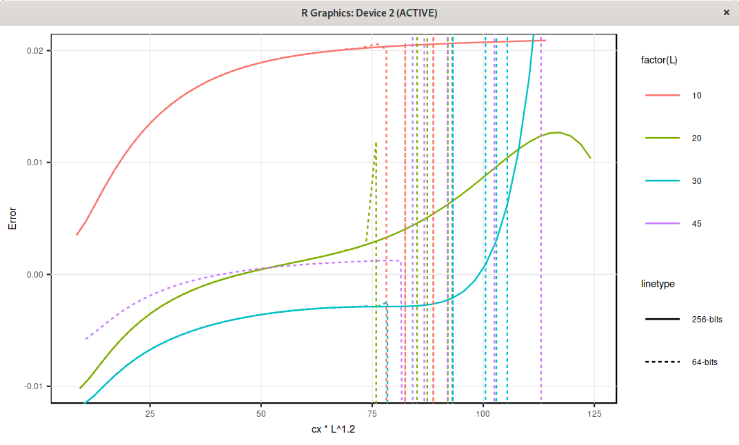
Error in price against the scaled shape parameter, for different grid sizes L, and 64 bits or 256 bits floats.
Here, the optimal shape parameter is around \( c = \frac{60}{L^{1.2}} \), corresponding to the flatter region, and the error actually seems to increase if the shape parameter is chosen too high with 256 bits floats. With 64-bits, it is not as clear since the system explodes.
Unfortunately, after all the hard work, from the results I got, I am not convinced that using a higher precision really helps that much my case. So I thought it would be interesting to give at least a feedback on…
Julia vs. Python
This is not going to be a comparison between Julia and Python in general. I am sure there exists already many great articles on Julia vs. XYZ language available on the internet. The below is more a “hands on Julia” from a numerical scientist point of view.
good
By default, no punctuation is required at the end of each sentence. If the sentence is executed directly in the REPL, the output is displayed. If it is embedded inside a function, the output is not displayed. This allows to quickly test some parts, by copy pasting pieces of a function in the REPL, and once it is ready, all the internal state is immediately hidden. I found this quite convenient, possibly better than Matlab, where an explicit semicolumn is required to remove the output.
Fast. Of course, it all depends on the point of reference, but compared to numpy, a simple RBF PDE solver port from numpy to julia ended up being 30% faster without even looking at optimization (for relatively small systems).
not great
Default linux packages from your distribution provider (Fedora 30 in my case) are broken. Even the special COPR repo version is broken. It is important to download the binary from julia.org website instead. How is it broken? It kept complaining it could not compile Arpack in my case, when I tried to use the package LinearAlgebra.
Not always clear which libraries to use. Python numpy or scipy are much bigger libraries and you can do a lot just with those. In Julia, you have packages for polynomial roots, statistical functions, linear algebra… This does not make it always clear which one to use.
Syntax is not as immediatly obvious as Python: to apply the max function elementwise on a vector minus a constant, you write something like “max.(S .- K, 0.0)”. If you write 0 instead of 0.0, it complains. If you forget a “.”, it complains with some not-so-obvious error message for the uninitiated. Thanksfully, there is stackoverflow and google to help. This may be very minor, since once you understand the right way, it becomes quite powerful. For example, in numpy, I had to use sometimes explicitely the .divide function to work on matrices elementwise. The “.” notation of Julia takes care more naturally of this.
The doc is not as polished as the one from numpy or scipy.
The “global” keyword is sometimes required when evaluating some loop in the REPL, but not if the loop is embedded inside a function. A minor annoyance, but this seems a bit awkward to me.
multiple precision performance
Now regarding the multiple precision arithmetic performance: the RBF solver is around 10x-60x slower with 256-bits floats (Arb library ArbField(256)) than with 64-bits floats (Julia Float64), depending on the size of the system to solve. On a specific setup, Julia BigFloat took 1400s while Arb took 16.7s on my problem. And Julia BigFloat is supposedly faster than python mpmath…
So clearly, the use of multiple precision makes RBF collocation not really practical. Now, without multiple precision, one can still achieve a reasonable accuracy on relatively small grids, for example a 50x50 grid. It becomes however quite challenging to increase the accuracy, as the computational cost evolves in \( O(L^6) \) for an LxL grid of points. Furthermore, I believe that some of the loss of accuracy is directly related to the non-smooth initial conditions that I use on my specific problem. This makes the RBF collocation not so competitive when compared to classic second order finite difference methods (on my problem), which allow for much denser discretization grids for a given computational cost.
I had to recode quite a bit around the Arb library, as it does not support many of Julia linear algebra concepts. For the curious, I also implemented the approx lu solver in Julia, based on the code of the Julia Nemo library, which interfaces with the C Arb library, but lacks the approx lu solver.
function approx_lu!(P::Generic.perm, luMat::arb_mat, x::arb_mat)
    r = ccall((:arb_mat_approx_lu, :libarb), Cint,
    (Ptr{Int}, Ref{arb_mat},  Ref{arb_mat}, Int),
    P.d, luMat, x, prec(base_ring(x)))
    r == 0 && error("Could not find $(nrows(x)) invertible pivot elements")
    P.d .+= 1
    return nrows(x)
end

function approx_solve_lu_precomp!(z::arb_mat, P::Generic.perm, luMat::arb_mat, y::arb_mat)
    r = ccall((:arb_mat_approx_solve_lu_precomp, :libarb), Nothing,
    (Ref{arb_mat}, Ptr{Int}, Ref{arb_mat},  Ref{arb_mat}, Int),
    z, P.d .- 1, luMat, y, prec(base_ring(y)))
    nothing
end