Exponential B-Spline Collocation and Julia Automatic Differentiation
New algorithms for polynomial stochastic collocation and exponential B-spline collocation are available now in my github repo. I had a few surprises while recreating those in Julia and using the forward automatic differentiation.
October 12, 2021
I just added the exponential B-spline collocation to produce a flexible arbitrage-free interpolation of implied-volatilities to the book related github repo. I had written the polynomial collocation before, at the request of a reader of my book. The polynomial collocation is often what you will want to use but it has a few drawbacks sometimes:
- It may not always fit well enough given the limited number of free-parameters.
- It sometimes produces artificial spikes in the extrapolation, even if the use of a specific regularization helps to address this.
- There is absorption at zero.
The exponential B-spline collocation offer as many parameters as anyone wants, avoids spikes (but also needs regularization in practice), and will map to the open interval \( (0, +\infty) \): no absorption to deal with. An alternative, that I actually explored, would be a B-spline collocation towards the lognormal distribution. In general, the alternative is not interesting, since it produces a worse fit, for the same reasons as with a polynomial, as described out there.
Compared to the reference paper, I had to make a few modifications:
- a different kind of regularization for real market data such the TSLA examples (use the difference in \(1/g’\) instead of \(g’’\), as the probability density depends on \(1/g’\)).
- a proper choice of the first B-spline coefficient, such that the theoretical forward does not explode. The first coefficient may be chosen arbitrarily as it is then adjusted to match the market forward price.
- some care with NaNs due to the interaction of the exponential and normal cumulative distribution functions. This also interplays with automatic forward differentiation.
- the use of knots at x instead of in the middle avoids some oscillations in the absence of any regularization term.
The third item is actually the trickiest one. Even though it is obvious after the facts, I did not think that forward automatic differentiation would lead to such subtle issues. While it is often not too difficult to deal with eventual NaNs in the evaluation of a given objective function (for example in \( e^{x} f(x) \) with \( \lim_{x \to \infty} e^{x} f(x) = 0 \) the exponential will go to infinity even though the result must be zero), it is much less obvious to think about what could go wrong with the forward differentiation. There are trivial examples such as:
using ForwardDiff
g(x) = sqrt(abs(x))
ForwardDiff.derivative(g, 0.0)
the function evaluation is well defined, but the function is not differentiable at 0. For differentiation to work, the following definition is required:
g(x) = x < 0 ? sqrt(abs(x)) : zero(x)But in my case, the differentiation happens over a non-trivial portion of code (and it’s actually amazing that it works most of the time without issues).
It does not seem to uncommon for people to fight NaNs due to automatic forward differentation, see for example this thread and related, or that one.
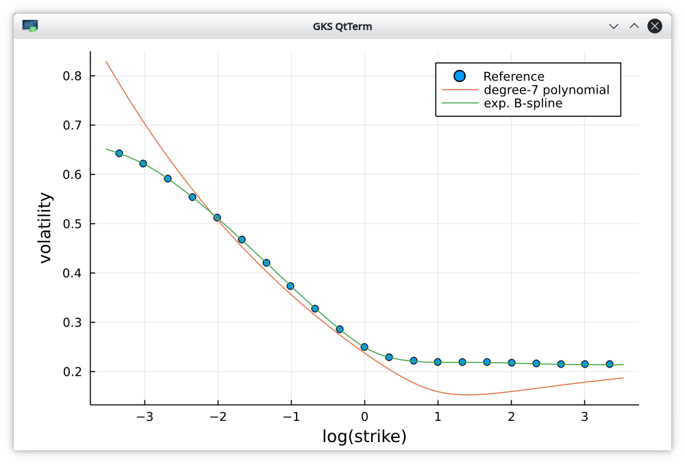
Implied volatilities on the extreme market data of Peter Jaeckel.
| Method | RMSE in implied vol % |
|---|---|
| Polynomial degree 7 | 5.099 |
| Exponential B-spline lambda=0 | 0.012 |
| Exponential B-spline lambda=1e-2 | 0.050 |
On real market data, it may be advantageous to use Gauss-Hermite nodes instead of the raw market implied nodes. With the same regularization (1e-2), and the same number of nodes, this leads to a very smooth implied density for the example of TSLA options of 18m maturity, much smoother than with the raw nodes without sacrifying too much accuracy. This is because the raw nodes are too close to each other when there are a lot of market observations and too far when there are few market observations.
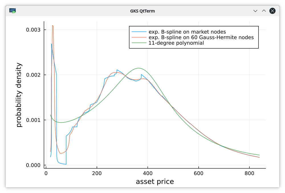
Implied probability density on TSLA option of maturity 18 months.
| Method | RMSE in implied vol % |
|---|---|
| Polynomial degree 7 | 1.31 |
| Polynomial degree 11 | 0.93 |
| Exponential B-spline lambda=0 | 0.35 |
| Exponential B-spline lambda=1e-2 | 0.36 |